

As I have expanded upon lengthily in this previous post, interference is a key phenomenon in quantum theory. In this post, we will see how it can be used to explain the existence of forces between certain objects, using the example of the electromagnetic force in particular.
The usual popular account of the quantum origin of forces rests on the notion of virtual particles. Basically, two charged particles are depicted as 'ice skaters' on a frictionless plane; they exchange momentum via appropriate virtual particles, i.e. one skater throws a ball over to the other, and both receive an equal amount of momentum imparted in opposite directions. This nicely explains repulsive forces, i.e. the case in which both skaters are equally charged. In order to explain attraction, as well, the virtual particles have to be endowed with a negative momentum, causing both parties to experience a momentum change in the direction towards the other. Sometimes, this is accompanied by some waffle about how this is OK for virtual particles, since they are not 'on-shell' (which is true, but a highly nontrivial concept to appeal to for a 'popular level' explanation).
In this post, after the introduction, I will not talk about virtual particles anymore. The reason for this is twofold: first, the picture one gets through the 'ice-skater' analogy is irreducibly classical and thus, obfuscates the true quantum nature of the process, leaving the reader with an at best misleading, at worst simply wrong impression. Second, and a bit more technically, virtual particles are artifacts of what is called a perturbation expansion. Roughly, this denotes an approximation to an actual physical process by means of taking into account all possible ways the process can occur, and then summing them to derive the full amplitude -- if you're somewhat versed in mathematical terminology, it's similar to approximating a function by means of a Taylor series. The crucial point is that the virtual particles are present in any term of this expansion, but the physical process does not correspond to any of those terms, but rather, to their totality. So the virtual-particles analogy can't give you the full picture.
Interference, on the other hand, can, or at least so I believe. In order to make this as self-contained as possible (though I would urge you to read the already-linked previous post), let's briefly review a few facts about interference.
Interference
Interference is a phenomenon present in waves. Waves can interfere constructively, destructively, or in various intermediate ways. In order to determine the interference of two waves, you simply superimpose their graphs, and add the amplitudes in the appropriate places. Consider these three different waves:
 |
| Fig. 1: Three waves. |
If they interfere, they give rise to this new waveform:
 |
| Fig. 2: Wave interference. |
As you can see, the waves reinforce one another in some places, and cancel each other out in others. For another picture, consider waves upon a surface of water: where a peak encounters another peak, they create a higher (as high as both peaks put upon one another) peak, while where a valley encounters another valley, there will be a deeper resulting valley; while if a peak meets a valley of an appropriate depth, flat sea may result.
Interference depends on the relative phase between the waves. If pictured on the x-axis, the phase denotes the shift of the waveform:
 |
| Fig. 3: Two waves, differing only in their phase. |
Plainly, the above to waves, if brought into superposition, will interfere completely destructively. The phase of a wave can be effectively depicted as an angle in the so-called phasor representation:
 |
| Fig. 4: Three waves, depicted by means of their phases and amplitudes. (Image credit: wikipedia.) |
The angle of the little arrows represent each wave's phase; their length their respective amplitudes. Adding the arrows produces a third arrow, representing the phase and amplitude of the wave resulting from their interference.
Now, you can associate a phase to each quantum state. As the state evolves in time, the phase rotates, as in the figure. Thus, quantum states can interfere with one another. This is demonstrated in Young's classical double slit experiment:
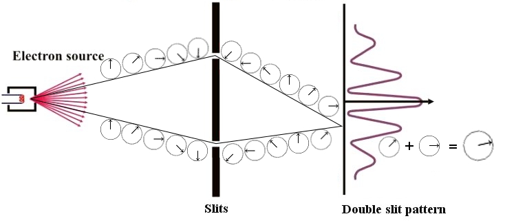 |
| Fig. 5: Double slit experiment with phases shown. |
I have indicated the evolution of the phase as each state propagates. In the end, the interference pattern is obtained by adding the phases, as shown. At the point where the two sample trajectories meet on the screen, constructive interference occurs, leading to a peak.
Phase Invariance
Another property of quantum mechanics is that it is invariant under arbitrary, global phase changes. Thus, global phase change is a symmetry of the theory. Symmetry is a very important concept in modern physics, perhaps even the most important one. Basically, a symmetry is something you do to a system such that it doesn't change observably.
In this post, we will be concerned with the symmetries of a very simple object, the circle. These are simply the rotations through an arbitrary angle: if I show you a circle, then tell you to close your eyes, do something to the circle, you will not be able to tell whether or not I have rotated it -- the circle still looks the same. (You can also reflect a circle through an arbitrary axis going through its center, but this will not concern us here.)
Symmetries form a mathematical object called a group. Roughly, this just means that you can compose symmetries in a certain way and have the composition be a symmetry again -- in the present case, subsequent rotation through 90° and 45° is equivalent to a single rotation through 135°. There exists an identity element, e, which corresponds to 'doing nothing' -- rotating through an angle of 0°, if you will. There is also the notion of an inverse element, i.e. an operation that undoes a previous one -- rotating by 45° rightwards, if you have previously rotated through 45° leftwards. Just to be complete, for technical reasons, we also require associativity -- mathematically, this is written as (R1 • R2) • R3 = R1 • (R2 • R3), and doesn't mean anything other than that it doesn't matter whether we first perform the rotations one and two, followed by three, or two and three, followed by one.
The particular group that describes the symmetries of the circle is aptly named the circle group, or, somewhat more opaque, U(1).
The phase invariance of quantum mechanics is then encapsulated in the statement that quantum mechanics has a global U(1)-invariance. To see this, let's look at what happens if we change the global phase in the double slit experiment:
 |
| Fig. 6: Interference with a global phase shift. |
Note that the absolute phases change -- by 90° --, but the relative phase, between the upper and lower path, stays the same. Thus, in the end, the amplitude, which determines the size of the peaks on the screen, is the same as before -- the global phase shift did not change the interference pattern.
Interlude: The Aharonov-Bohm Effect
Now, we've got the machinery in place to talk about another 'weird' consequence of quantum theory: the Aharonov-Bohm effect, in which the presence of an electromagnetic potential alters the relative phases of quantum states. The setup is a slight modification of the double slit experiment:
 |
| Fig. 7: Aharonov-Bohm setup. Note the shifted interference pattern. |
Basically, we introduce a solenoid (the circle), idealized to be infinitely long, into the setup. This solenoid introduces a certain electromagnetic potential, denoted Aμ. As a consequence, we observe a shift in the interference pattern (the effect of the potential Aμ is shown as a change in speed in the evolution of the phases.)
This is quite curious! Classically, one would not expect an effect to occur. This is because the magnetic field B outside of an infinite solenoid is equal to zero (it is only nonzero inside), and thus, there is no influence by the field on the particles going around the solenoid.
I will not, at this point, attempt to provide an explanation of the Aharonov-Bohm effect. We will simply take it as an experimental datum to be incorporated into our theory, and proceed.
Local Phase Changes
After this, let's consider what happens if we change the phase not globally, but locally, i.e. apply our phase shift only to one of the beams. Quantum mechanics is not invariant under such a transformation; it is not a symmetry of the theory. Thus, the interference pattern changes:
 |
| Fig. 8: Non-invariance under local phase transformations. Again, note the shifted interference pattern. |
But what if, for whatever reason, we want a theory invariant under local U(1) phase changes? Well, we can use the Aharonov-Bohm effect to our advantage, and introduce an appropriate electromagnetic potential such that the effect of the local phase change is exactly cancelled, and the original interference pattern is recovered:
 |
| Fig. 9: Introducing an electromagnetic potential restores the original interference pattern. |
Thus, if we want a theory that is invariant under local U(1) transformations, we must necessarily include an electromagnetic potential! And with the potential, we get the rest of electromagnetism, as well. (For the mathematically inclined, the electromagnetic potential I have introduced is a four component quantity Aμ = (cΦ, A1, A2, A3), where Φ denotes the electric (scalar) potential, the gradient of which is the electric field E, and A = (A1, A2, A3) denotes the magnetic (vector) potential, the curl of which is the magnetic field B.)
This is an amazing result -- most of the phenomena we experience in everyday life (excluding those related to gravity) are a result of the electromagnetic force: not just obvious things like lighting, TVs and other electric appliances, but also the fact that you can't move through walls or fall to the floor, every optical effect etc.
That merely postulating local U(1) invariance serves to explain things as majestic and magnificent as rainbows and lightning storms speaks to the great power of the principle.
Test case: Electrostatic Repulsion
To this point, this all probably seems rather abstract: with careful juggling of phase transformations and suitably introduced potentials, one can ensure the invariance of interference patterns on a screen. This does not seem to have much to do with what we ordinarily think of as electromagnetism. So let's consider a paradigmatic example, the electrostatic interaction between two point charges (for instance, electrons) and see how our new understanding sheds light on the matter.
First, another reminder. Previously, I've told you how the speed of the phase change of a particle dictates the path it takes through spacetime. To briefly recap, consider not just a double, but triple, quadruple, and so on, slit experiment, with not just one, but many perforated screens in between.
Clearly, at every point, the amplitudes of all quantum states have to be summed, according to their respective phases. This is the kernel of the path integral formulation of quantum mechanics -- imagine infinitely many slits and infinitely many screens; what you get is empty space, since at every point in space, there will be a slit. Thus, in order to calculate the propagation of a particle through space, you have to sum up the amplitudes to propagate through every point in space, according to the relative phases. In this way, there will emerge a most likely path for the particle to take, and this path will be the classical path -- in empty, flat space, a straight line.
Test case: Electrostatic Repulsion
To this point, this all probably seems rather abstract: with careful juggling of phase transformations and suitably introduced potentials, one can ensure the invariance of interference patterns on a screen. This does not seem to have much to do with what we ordinarily think of as electromagnetism. So let's consider a paradigmatic example, the electrostatic interaction between two point charges (for instance, electrons) and see how our new understanding sheds light on the matter.
First, another reminder. Previously, I've told you how the speed of the phase change of a particle dictates the path it takes through spacetime. To briefly recap, consider not just a double, but triple, quadruple, and so on, slit experiment, with not just one, but many perforated screens in between.
 |
| Fig. 10: Multi-slit experiment. |
Clearly, at every point, the amplitudes of all quantum states have to be summed, according to their respective phases. This is the kernel of the path integral formulation of quantum mechanics -- imagine infinitely many slits and infinitely many screens; what you get is empty space, since at every point in space, there will be a slit. Thus, in order to calculate the propagation of a particle through space, you have to sum up the amplitudes to propagate through every point in space, according to the relative phases. In this way, there will emerge a most likely path for the particle to take, and this path will be the classical path -- in empty, flat space, a straight line.
This occurs because the more a path deviates from this classical path, the faster the phase of the particle following that path changes; but this means that on these non-classical paths, the particle grows ever more likely to destructively interfere with itself the more the path deviates from the classical one. Thus, the classical path emerges as the most likely one.
The 'speed' of the particle's phase evolution is given by a quantity known as the action, which depends on the difference between its kinetic and potential energy. The greater the action, the faster the phase rotates, the less likely the path is to be taken. Thus, the principle of least action emerges from quantum mechanics.
Now let us look at the aforementioned case of two like charges, say electrons. For simplicity, assume that one, the leftmost, is fixed to its position by some means.
 |
| Fig. 10: Two charges. Which of the possible paths will the right one take? |
Note that in the figure, time runs upward, space to the right; so any particle stationary in space will follow a straight upwards-directed trajectory in the plane, as indicated for the left charge. Our task is now to determine the path of the second, free, charge from what we have learned so far. Will it be attracted to the first (path (1))? Will it remain stationary, as well (path (2))? Or will it be repulsed, and if so, how much (paths (3) and (4))?
To answer this question, we need to take a closer look at the quantity I have previously introduced, the action. For a particle following a certain path between the times t1 and t2, the action can be written in the form S = (T - V)(t1 - t2), where T and V denote the average kinetic and potential energy, respectively. Plainly, this increases with increasing kinetic energy -- which is a good thing, otherwise, the action could always be minimized by going faster, so everything in the universe would spontaneously accelerate without bound for no good reason. So Newton was on a good track with his first law -- things on which no force acts indeed don't accelerate.
Now for the potential energy. Since we are in an electrostatic setup, we can simply consider the electric potential Φ. An electron in a potential Φ has a potential energy V = -eΦ. Φ gets bigger the closer the two electrons are together; thus, moving them apart lowers the potential, and with it, the action (note the all-important minus sign!). Thus, there is a 'sweet spot' for the action: it will be minimal on paths that take the second electron farther away from the first one -- but not too fast, or otherwise, the kinetic energy gets too large!
Qualitatively, this thus nets us the immediate conclusion that like charges repel. Just as immediately, by exchanging the minus sign I just drew your attention to with a plus, corresponding to exchanging the left, negative charge by a positive one (say a positron), we obtain that opposite charges attract.
I should, perhaps, loose a few words on what, exactly, I mean by 'charge'. Essentially, the charge of an object sets a 'speed scale' for the rotation of its phase: the higher the charge, the faster the rotation. Thus, more highly charged particles react more strongly to electromagnetic fields (and uncharged ones don't react at all) -- which is as it should be. Charge thus determines the strength of the coupling to the electromagnetic potential.
Recap
Since we have come quite a way from where we started, it is useful to take a moment and recapitulate what brought us here. We started out with the phase invariance of quantum mechanics. The Aharonov-Bohm effect taught us that changes in local phase, i.e. changes by local U(1) transformations, can be countered by the introduction of an electromagnetic potential. Thus, we obtained a theory invariant under local phase changes. This theory, as we have seen, successfully predicts the basic principles of electromagnetism, such as attraction/repulsion of opposite/like charges. In fact, it is easy to go a step further: the least action principle straightforwarldy implies Newton's second law, F = ma; in this particular case, F = -dΦ/dx = -eE, and thus, the Lorentz force law follows. (And since we could have equally well undertaken these considerations for the other charge, Newton's third law follows just as well.) It is remarkable that all this can be deduced from quantum interference and the simple symmetry principle we have introduced!
However, using the Aharonov-Bohm effect threatens the argument with circularity: it uses a dependence of the phase on the electromagnetic potential to show that particles react to the electromagnetic potential. Understanding this as an experimental input removes the circularity, however, the argument can be made fully independently, though at the expense of a little math. Basically, in order to insure invariance under local U(1) transformations, we find that we must modify our notion of differentiation; in order to do so, we must again introduce a quantity that has the effect of again removing the position-dependence from the theory. Mathematically, this quantity is known as a connection, and physically, it turns out to be just the electromagnetic potential Aμ.
Thus, the argument is complete in itself, and all the input that is needed is the local U(1) invariance.
What is Aμ?
Up to now, I have been cagey on the nature of the mysterious quantity we needed to introduce into the theory to insure invariance. The reason for this is that it's not easy to grasp. Physically, quantities like Aμ are called 'gauge potentials', for historical reasons. The defining characteristic of gauge potentials is that they're arbitrary to a certain degree -- meaning, there exists more than one choice of Aμ that lead to the same electric and magnetic fields, which, after all, are the only things we observe physically. So it seems as if Aμ can be little more than a bookkeeping device, and classically, that is indeed the way it is most commonly treated.
However, as we have already seen, in quantum mechanics, the potential takes center stage. Electrons don't couple to magnetic or electric fields, they couple directly to the potential. Furthermore, in the Aharonov-Bohm setup, an effect is observed even though no particle ever had a non-negligible amplitude to be in any region where the electromagnetic field differs from zero.
For the moment, we will leave the question of the 'reality' of the gauge potential aside, and instead consider its properties. In quantum field theory, each field is accompanied by a particle, corresponding to an excitation of the field: picture the field as a three-dimensional array of points, connected with springs; if you pull on one of the points, and then release it, it will start to oscillate, causing nearby points to oscillate as well, and so on. This excitation corresponds to the particle.
So, what's the particle associated to Aμ? First of all, we note that the electromagnetic interaction appears to be infinite in range. This means that the particle must be massless, due to an elementary consideration involving the energy-time uncertainty principle, ΔEΔt ~ h, where h is Planck's constant. The energy of the particle, given by the relativistic mass-energy relationship, is mc², and thus, it can't exist as an intermediary ('virtual') state for a time longer than h/mc², during which it can propagate a distance of at most hc/mc² (the heuristic nature of this argument makes me not worry about factors of 2π and such). Thus, only massless particles can mediate forces across infinite distances.
Second, it is itself electrically neutral, at least to a high degree of certainty. If that weren't the case, it would couple to itself strongly, leading to novel features, like possibly confinement (confinement is a property of the strong interactions, where the force mediating particles -- the gluons -- indeed carry appropriate charges themselves; effectively, its effect is to 'shield' quarks from direct observation. Since we observe electrons directly, we know the electromagnetic interaction is not confining.).
Third, its spin is 1. This essentially follows because Aμ is a vector field; scalar fields (just numbers at certain spacetime points) lead to spin zero particles, 2-tensor fields (like the metric of general relativity, gμν) have a spin of two, etc.
Thus, the particle, or field quantum, of the electromagnetic potential is massless, chargeless, and has spin 1 (and is thus a boson). That particle is what we normally call the photon. So this, too, comes out of our simple requirement of local U(1) symmetry -- let there be light, indeed.
Postscript -- Other Forces
Besides the electromagnetic force, there exist (at least) three more forces in nature, which combined serve to explain the full multitude of phenomena hitherto observed (or close to that, anyway). These forces are the two nuclear forces, called 'weak' and 'strong' in a very down-to-the-point manner, and gravity. The strong force keeps the nuclei together and thus, ensures the stability of matter; the weak force is responsible for nuclear processes, and among other things, makes the sun shine. Gravity, of course, keeps our feet on the ground -- perhaps the most important of the three.
For the two nuclear forces, a story similar to the one I have just related can be told. The major difference is in the symmetry groups -- the weak force requiring local SU(2) symmetry, which is related to the symmetries of a three-dimensional sphere, while the strong force is described by a SU(3) gauge theory called quantum chromodynamics. Both accounts differ from the simple one I have given in this post in some ways: one difference is that the symmetry transformations no longer commute, i.e. doing one transformation, then the other, is not the same as doing them in reversed order. This is not that unusual: rotations in three dimensions behave the same way. Take any object, such as a book, and rotate it first through one axis, then through another; put it back into its original state, and do the rotations in inverse order, and you will generally get a different final orientation.
Both forces also have their own quirks. For instance, there is, strictly speaking, no theory of the weak interaction on its own; instead, it is described in a unified way together with the electromagnetic interaction, via the so-called electroweak theory, based on the direct product of the groups SU(2) and U(1), SU(2) x U(1) -- we speak of a unified theory in this case. In order to get the usual phenomenology from the theory, this symmetry has to be broken, which is the main job of the recently-discovered Higgs field (the mass-giving aspect comes in almost accidentally). An added complication is that the U(1) responsible for electromagnetism is not the straightforward one in SU(2) x U(1), but actually a different subgroup.
The strong force, on the other hand, shows the peculiar phenomenon known as confinement -- since its gauge bosons carry the charges appropriate to the theory themselves (conventionally denoted as the three colors red, green, and blue), they conspire, via self-interaction, to hide the explicit workings on the quark level from view, making only color-neutral ('white') states observable.
Apart from these differences, though, the conceptual structures of these theories are as described in this post, and their conceptual similarity has led them to be subsumed in one immensely successful meta-theory called simply the standard model, based on the gauge group SU(3) x SU(2) x U(1). This is, however, not a genuine unification in the way the electroweak theory is; thus, the quest for a more fundamental, and perhaps theoretically more appealing so-called grand unified theory (GUT), the basic strategy for which is to embed the standard model group in some larger group, such as SU(5), SO(10) or the exceptional E(6), is ongoing.
Gravity, on the other hand, seems much more reluctant to join into the reign of the other forces. Our understanding of gravity is essentially macroscopic, and so far, it has resisted all attempts to be brought in line with the quantum paradigm. While there are tantalizing similarities with the gauge structure of the other forces, every attempt to join them on traditional terms so far is either inconclusive, or has ended in outright failure. Thus, the quest for quantum gravity -- and the even larger endeavor to unify all the forces into one single theory of everything -- remains today unfulfilled, and the greatest challenge for physics.
http://www.academia.edu/7347240/Our_Cognitive_Framework_as_Quantum_Computer_Leibnizs_Theory_of_Monads_under_Kants_Epistemology_and_Hegelian_Dialectic
AntwortenLöschenVery well written. Thank you!
AntwortenLöschen